MISC
Gaussian process is a non-parameter model (fewer hyperparameters than neural network, and easy to implement). The computational bottleneck is the matrix inversion ($O(N_\text{samples}^3)$). Predicting covariances is more time consuming than predicting mean values (check the option to only predict mean values in different packages). When including derivative observations, predicting covariances is very slow and often not necessary.
Basic
For a given set of finite data points, there are potentially infinitely many functions that fit the data.
We need to make assumptions about the underlying functions, otherwise the predicted function (colored dashed lines) could be wild.
Gaussian processes is a powerful method to solve this fitting problem by assigning a probability to each of colored dashed line.
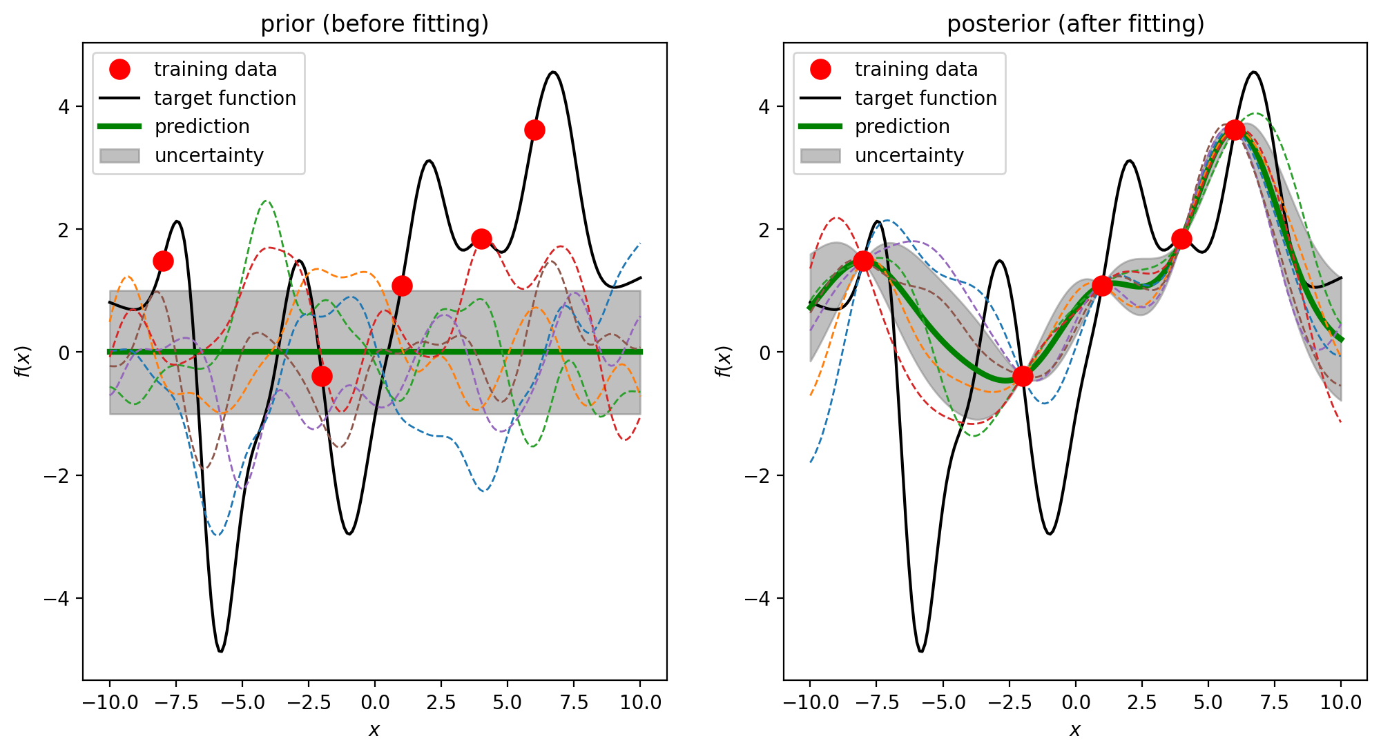
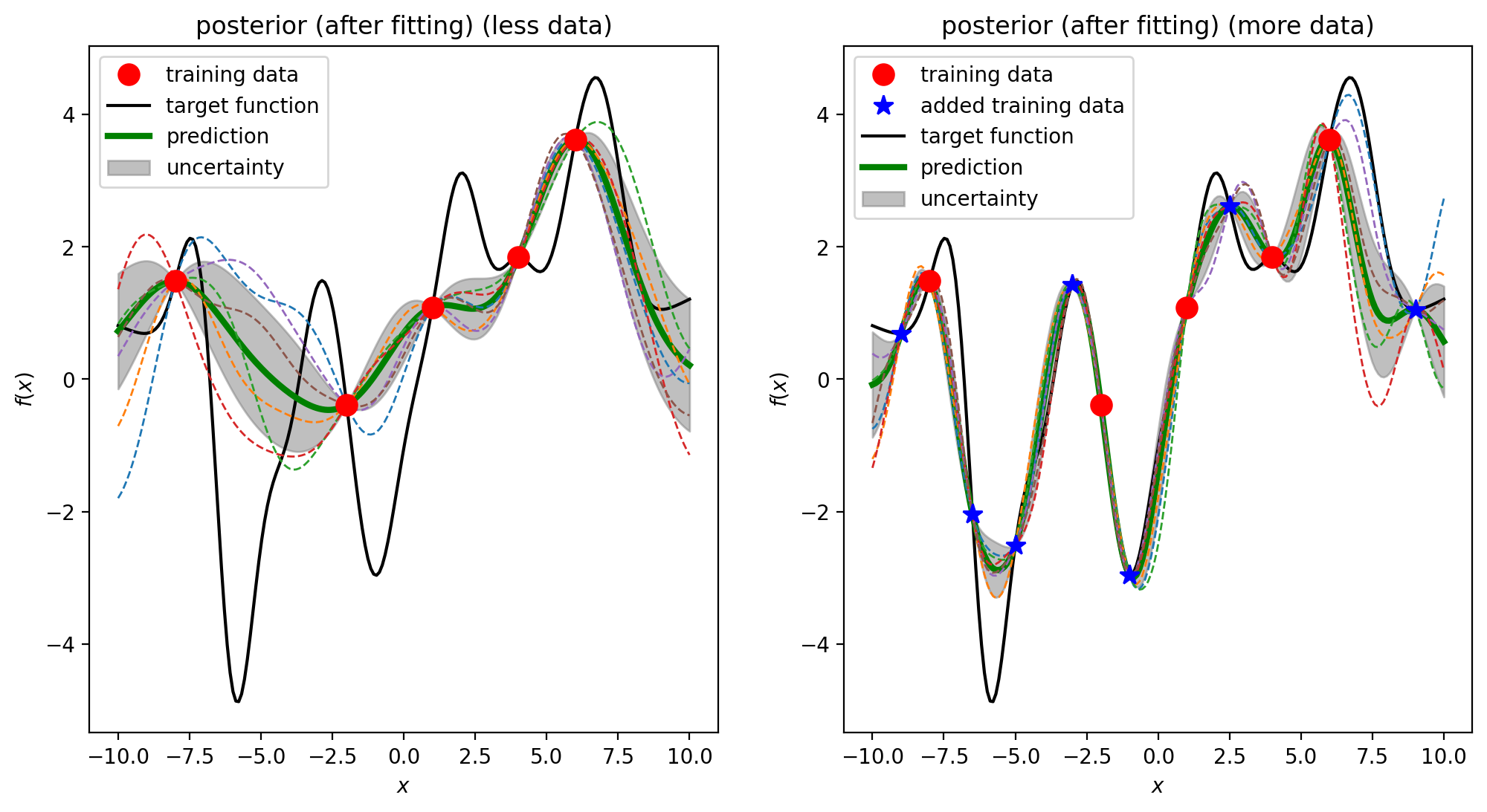
GP can predict the value of an unknown data and the confidence (uncertainty) about how much we can trust this value. The uncertainty directs us to add new data to the training set and presumably improves the prediction.
conditioning: the probability of one variable depending on another variablemarginalizationandconditioningyield a modified Gaussian distribution- correlation intuition: imagine a earthquake is attacking many cities including ABC. The distance between City A and City B is closer than the distance between City A and City C ($d(A, B) < d(B, C)$). The intensity each city feels is defined as $I$. The $I _ A$ and $I _ B$ has higher correlation, and $I _ A$ and $I _ C$ has lower correlation. If we can only detect $I _ A$ at this moment and want to predict $I _ B$ and $I _ C$, we will be more certain about the prediction on City B than City C.
Functional view
We have a collection of input $\textbf{X} = [ \textbf{x} _ 1, \textbf{x} _ 2, \dots, \textbf{x} _ n ]^T \in \R^{n \times d}$ where $n$ is the number of training data and $d$ is the dimension of the feature. The input space $\textbf{x}_i$ is infinite and continuous in space with a fixed number of components ($\textbf{x} _ i = [x(1), x(2), \dots, x(d)]$). The corresponding output is $\textbf{y} = [y _ 1, y _ 2, \dots, y _ n]^T \in \R^{n \times 1}$.
The goal is to find the mapping $f$ from $\textbf{x}$ to $y$ which corresponds to $y = f(\textbf{x})$ in a noise-free case. We suppose $f$ is a gaussian process which is defined by its mean function $m(\textbf{x})$ and covariance function $k(\textbf{x}, \textbf{x}^\prime)$ $$ \begin{aligned} m(\textbf{x}) &= \mathbb{E}(f(\textbf{x})) \\ k(\textbf{x}, \textbf{x}^\prime) &= \mathbb{E}[(f(\textbf{x}) - m(\textbf{x}))(f(\textbf{x}^\prime) - m(\textbf{x}^\prime))] \end{aligned} $$ If we want to predict outputs at $m$ locations ($\textbf{x} _ {\ast 1}, \textbf{x} _ {\ast 2}, \dots, \textbf{x} _ {\ast m}$) $$ \underbrace{f(\textbf{x} _ 1), \dots, f(\textbf{x} _ n)} _ {\text{training points}}, \underbrace{f(\textbf{x} _ {\ast 1}), \dots, f(\textbf{x} _ {\ast m})} _ {\text{test points}} \sim N(0, \sum) $$
where
$$ \begin{aligned} \sum &= \left[ \begin{array}{ccc|c} k(\textbf{x} _ 1, \textbf{x} _ 1) & \dots & k(\textbf{x} _ 1, \textbf{x} _ n) & k(\textbf{x} _ 1, \textbf{x} _ {\ast 1}) & \dots & k(\textbf{x} _ 1, \textbf{x} _ {\ast m}) \\ \vdots & & \vdots & \vdots & & \vdots \\ k(\textbf{x} _ n, \textbf{x} _ 1) & \dots & k(\textbf{x} _ n, \textbf{x} _ n) & k(\textbf{x} _ n, \textbf{x} _ {\ast 1}) & \dots & k(\textbf{x} _ n, \textbf{x} _ {\ast m}) \\ \hline k(\textbf{x} _ {\ast 1}, \textbf{x} _ 1) & \dots & k(\textbf{x} _ {\ast 1}, \textbf{x} _ n) & k(\textbf{x} _ {\ast 1}, \textbf{x} _ {\ast 1}) & \dots & k(\textbf{x} _ {\ast 1}, \textbf{x} _ {\ast m}) \\ \vdots & & \vdots & \vdots & & \vdots \\ k(\textbf{x} _ {\ast m}, \textbf{x} _ 1) & \dots & k(\textbf{x} _ {\ast m}, \textbf{x} _ n) & k(\textbf{x} _ {\ast m}, \textbf{x} _ {\ast 1}) & \dots & k(\textbf{x} _ {\ast m}, \textbf{x} _ {\ast m}) \end{array} \right] \\ &= \left[ \begin{array}{c|c} K(X, X) & K(X, X_\ast) \\ \hline K(X_\ast, X) & K (X _ \ast X _ \ast) \end{array} \right] \end{aligned} $$
Derivatives
Suppose we have atoms A and B in the system with a total energy E, the force acting on atom A is $\textbf{f} _ A = [f _ {Ax}, f _ {Ay}, f _ {Az}]$ and similarity $\textbf{f} _ B = [f _ {Bx}, f _ {By}, f _ {Bz}]$. The output vector for this system is expanded as $\textbf{y} = [E, f _ {Ax}, f _ {Ay}, f _ {Az}, f _ {Bx}, f _ {By}, f _ {Bz}]$
Brief (only in markdown)
Input matrix $\textbf{X} \in \R ^ {N \times D}$ contains the structure information of $N$ structures and the $i$th structure is represented as a $D$ dimensional feature vector $\textbf{x} ^ {(i)} = [x ^ {(i)} _ 1, x ^ {(i)} _ 2, \cdots, x ^ {(i)} _ D]$. In the cartesisan coordinates, the dimension of feature vector $D = 3 \times N_{\text{atoms}}$.
$$ \textbf{X} = \left[ \begin{array}{cccc} \textbf{x} ^ {(1)} \\ \textbf{x} ^ {(2)} \\ \cdots \\ \textbf{x} ^ {(N)} \end{array} \right] = \left[ \begin{array}{ccccc} x ^ {(1)} _ 1 & x ^ {(1)} _ 2 & x ^ {(1)} _ 3 & \cdots & x ^ {(1)} _ D \\ x ^ {(2)} _ 1 & x ^ {(2)} _ 2 & x ^ {(2)} _ 3 & \cdots & x ^ {(2)} _ D \\ \vdots & \vdots & \vdots & \ddots & \vdots \\ x ^ {(N)} _ 1 & x ^ {(N)} _ 2 & x ^ {(N)} _ 3 & \cdots & x ^ {(N)} _ D \end{array} \right] $$
The output matrix $\textbf{y} \in \R ^ {N \times 1}$ includes energies of $N$ structures $$ \textbf{y} = \left[ \begin{array}{cccc} y ^ {(1)} \\ y ^ {(2)} \\ \cdots \\ y ^ {(N)} \end{array} \right] $$ The goal is to find the mapping $f$ from $\textbf{x}$ to $y$ which corresponds to $y = f(\textbf{x}) + \epsilon$ and $\epsilon$ is the noise. We suppose $f$ is a gaussian process which is defined by its mean function $m(\textbf{x})$ and covariance function $k(\textbf{x}, \textbf{x}^\prime)$ $$ \begin{aligned} m(\textbf{x}) &= \mathbb{E}(f(\textbf{x})) \\ k(\textbf{x}, \textbf{x}^\prime) &= \mathbb{E}[(f(\textbf{x}) - m(\textbf{x}))(f(\textbf{x}^\prime) - m(\textbf{x}^\prime))] \end{aligned} $$ Then we can write the gaussian process as $$ f(\textbf{x}) \sim GP\Big(m(\textbf{x}), k(\textbf{x}, \textbf{x}^\prime)\Big) $$
A common choice of the covariance function is the squared exponential function. $$ k(\textbf{x}, \textbf{x}^\prime) = \sigma ^2 \text{exp} (- \dfrac{d(\textbf{x}, \textbf{x}^\prime) ^ 2}{2 l ^2}) $$ If we have a test point $\textbf{x} ^ \star$ and want to predict its energy. The joint distribution of the observed target values and the function values at the test location $\textbf{x} ^ \star$ is
$$ \left[ \begin{array}{cccc} \textbf{y} \\ f(\textbf{x} ^ \star) \end{array} \right] \sim N \Bigg[ \begin{array}{cccc} m(\textbf{X}) \\ m(\textbf{X} ^\star) \end{array} , \begin{array}{cccc} K(\textbf{X}, \textbf{X}) + \sigma ^ 2 _ N \textbf{I} & K(\textbf{X}, \textbf{X} ^ \star) \\ K(\textbf{X} ^ \star, \textbf{X}) & K(\textbf{X} ^ \star, \textbf{X} ^ \star) \end{array} \Bigg] $$
where the covariance matrix is
$$ \Sigma = \left[ \begin{array}{cccc} K(\textbf{X}, \textbf{X}) + \sigma ^ 2 _ N \textbf{I} & K(\textbf{X}, \textbf{X} ^ \star) \\ K(\textbf{X} ^ \star, \textbf{X}) & K(\textbf{X} ^ \star, \textbf{X} ^ \star) \end{array} \right] = \left[ \begin{array}{ccc|c} k(\textbf{x} ^ {(1)}, \textbf{x} ^ {(1)}) + \sigma ^ 2 _ N & \dots & k(\textbf{x} ^ {(1)}, \textbf{x} ^ {(n)}) & k(\textbf{x} ^ {(1)}, \textbf{x} ^ {\ast }) \\ \vdots & \ddots & \vdots & \\ k(\textbf{x} ^ {(n)}, \textbf{x} ^ {(1)}) & \dots & k(\textbf{x} ^ {(n)}, \textbf{x} ^ {(n)}) + \sigma ^ 2 _ N & k(\textbf{x} ^ {(n)}, \textbf{x} ^ {\ast }) \\ \hline k(\textbf{x} ^ {\ast }, \textbf{x} ^ {(1)}) & \dots & k(\textbf{x} ^ {\ast}, \textbf{x} ^ {(n)}) & k(\textbf{x} ^ {\ast }, \textbf{x} ^ {\ast }) \\ \end{array} \right] \\ $$
The prediction is based on Bayes' theorem $P(A|B) = \dfrac{P(A, B)}{P(B)}$. The predicted function value (energy, even though $y$ and $f$ has different meanings in GP, I just use the following notation for simplify) and its covariance are $$ \begin{aligned} y ^ \star_ {\text{pred}} = \bar{f}(\textbf{x} ^ \star) &= \underbrace{ \underbrace{m(\textbf{X} ^\star)} _ {\text{prior}} + K(\textbf{X} ^ \star, \textbf{X}) \Big[ K(\textbf{X}, \textbf{X}) + \sigma ^ 2 _ N \textbf{I} \Big] ^ {-1} \Big(\textbf{y} - m(\textbf{X}) \Big) } _ {\text{posterior}} \
\text{cov} (\textbf{x} ^ \star) &= K(\textbf{X} ^ \star, \textbf{X} ^ \star) - K(\textbf{X} ^ \star, \textbf{X}) \Big[ K(\textbf{X}, \textbf{X}) + \sigma ^ 2 _ N \textbf{I} \Big] ^ {-1} K(\textbf{X} , \textbf{X} ^ \star)
\end{aligned} $$ One can also predict the force on each atom by only training on energies. This is how GOFEE predicts the force. The predicted force component on $i$th atom along $\alpha$ axis is $$ - g ^ \star _ {i, \alpha} = - \sum ^ {N_ \text{features}} _ j \underbrace{\dfrac{\partial y ^ \star_ {\text{pred}}}{ \partial F_j}} _ \text{from GPR} \overbrace{\dfrac{\partial F_j}{ \partial R_{i \alpha}}} ^ \text{from features} $$ Such a method relies on either analytical gradients or automatic gradient implementations in both GPR and feature calculations.
training on forces
If we want train on both energies and forces. The output matrix should be expanded from $\textbf{y} \in \R ^ {N \times 1}$ to $\textbf{y} \text{ext} \in \R ^ {N \times (1 + 3 N \text{atoms})}$ which includes $3 N_ \text{atoms}$ force components in addition to energy.
$$ \textbf{y} = \left[ \begin{array}{cccc} y ^ {(1)} \ y ^ {(2)} \ \cdots \ y ^ {(N)} \end{array} \right] \rArr \textbf{y} _ \text{ext} = \left[ \begin{array}{cccccc} y ^ {(1)} & g ^ {(1)} _ {1,x} & g ^ {(1)} _ {1,y} & g ^ {(1)} _ {1,z} & \cdots & g ^ {(1)} _ {N_ \text{atoms},x} & g ^ {(1)} _ {N_ \text{atoms},y} & g ^ {(1)} _ {N_ \text{atoms},z}\ y ^ {(2)} & g ^ {(2)} _ {1,x} & g ^ {(2)} _ {1,y} & g ^ {(2)} _ {1,z} & \cdots & g ^ {(2)} _ {N_ \text{atoms},x} & g ^ {(2)} _ {N_ \text{atoms},y} & g ^ {(2)} _ {N_ \text{atoms},z}\ \vdots & \vdots & \vdots & \vdots & \ddots & \vdots & \vdots & \vdots \ y ^ {(N)} & g ^ {(N)} _ {1,x} & g ^ {(N)} _ {1,y} & g ^ {(N)} _ {1,z} & \cdots & g ^ {(N)} _ {N_ \text{atoms},x} & g ^ {(N)} _ {N_ \text{atoms},y} & g ^ {(N)} _ {N_ \text{atoms},z}\ \end{array} \right] $$
In GP-NEB paper (O.-P. Koistinen, F.B. Dagbjartsdóttir, V. Ásgeirsson, A. Vehtari, and H. Jónsson, J. Chem. Phys. 147, 152720 (2017). ) $$ \textbf{y} = \left[ \begin{array}{cccc} y ^ {\color{red}(1)} \ y ^ {\color{green}(2)} \ \cdots \ y ^ {\color{yellow}(N)} \end{array} \right] \rArr \textbf{y} _ \text{ext} = \left[ \begin{array}{cccc} y ^ {\color{red}(1)} \ y ^ {\color{green}(2)} \ \vdots \ y ^ {\color{yellow}(N)} \ g ^ {\color{red}(1)} _ {1,x} \ g ^ {\color{green}(2)} _ {1,x} \ \vdots \ g ^ {\color{yellow}(N)} _ {1,x} \ g ^ {\color{red}(1)} _ {1,y} \ g ^ {\color{green}(2)} _ {1,y} \ \vdots \ g ^ {\color{yellow}(N)} _ {1,y} \ g ^ {\color{red}(1)} _ {N,z} \ g ^ {\color{green}(2)} _ {N,z} \ \vdots \ g ^ {\color{yellow}(N)} _ {N,z} \ \end{array} \right] \in \R ^ {N(1 + 3N_{\text{atoms}}) \times 1}
\rArr \textbf{y} _ \text{ext} = \left[ \begin{array}{cccc} y ^ {\color{red}(1)} \ y ^ {\color{green}(2)} \ \vdots \ y ^ {\color{yellow}(N)} \ \hline g ^ {\color{red}(1)} _ {1} \ g ^ {\color{green}(2)} _ {1} \ \vdots \ g ^ {\color{yellow}(N)} _ {1} \ \hline g ^ {\color{red}(1)} _ {2} \ g ^ {\color{green}(2)} _ {2} \ \vdots \ g ^ {\color{yellow}(N)} _ {2} \ \hline g ^ {\color{red}(1)} _ {D} \ g ^ {\color{green}(2)} _ {D} \ \vdots \ g ^ {\color{yellow}(N)} _ {D} \ \end{array} \right] \in \R ^ {N(1 + D) \times 1} $$
The next step is to expand the covariance matrix which is only related with input features.
$$ \begin{aligned}
K(\textbf{X}, \textbf{X} ^\prime) &= \left[ \begin{array}{ccc} k(\textbf{x} ^ {(1)}, \textbf{x} ^ {(1)}) & k(\textbf{x} ^ {(1)}, \textbf{x} ^ {(2)}) & \dots & k(\textbf{x} ^ {(1)}, \textbf{x} ^ {(N^\prime)}) \ k(\textbf{x} ^ {(2)}, \textbf{x} ^ {(1)}) & k(\textbf{x} ^ {(2)}, \textbf{x} ^ {(2)}) & \dots & k(\textbf{x} ^ {(2)}, \textbf{x} ^ {(N^\prime)}) \ \vdots & \ddots & \vdots & \ k(\textbf{x} ^ {(N)}, \textbf{x} ^ {(1)}) & k(\textbf{x} ^ {(N)}, \textbf{x} ^ {(2)}) & \dots & k(\textbf{x} ^ {(N)}, \textbf{x} ^ {(N^\prime)}) \ \end{array} \right] \in \R ^ {N \times N^\prime} \
K_\text{ext}(\textbf{X}, \textbf{X} ^\prime)
&=
\left[
\begin{array}{c|cc}
K(\textbf{X}, \textbf{X} ^\prime) &
\dfrac{\partial K(\textbf{X}, \textbf{X} ^\prime)}{\partial x_1^\prime} &
\dfrac{\partial K(\textbf{X}, \textbf{X} ^\prime)}{\partial x_2^\prime} &
\dots &
\dfrac{\partial K(\textbf{X}, \textbf{X} ^\prime)}{\partial x_D^\prime}
\
\hline
\dfrac{\partial K(\textbf{X}, \textbf{X} ^\prime)}{\partial x_1} &
\dfrac{\partial ^2 K(\textbf{X}, \textbf{X} ^\prime)}{\partial x_1 \partial x_1^\prime} &
\dfrac{\partial ^2 K(\textbf{X}, \textbf{X} ^\prime)}{\partial x_1 \partial x_2^\prime} &
\dots &
\dfrac{\partial ^2 K(\textbf{X}, \textbf{X} ^\prime)}{\partial x_1 \partial x_D^\prime} \
\dfrac{\partial K(\textbf{X}, \textbf{X} ^\prime)}{\partial x_2} &
\dfrac{\partial ^2 K(\textbf{X}, \textbf{X} ^\prime)}{\partial x_2 \partial x_1^\prime} &
\dfrac{\partial ^2 K(\textbf{X}, \textbf{X} ^\prime)}{\partial x_2 \partial x_2^\prime} &
\dots &
\dfrac{\partial ^2 K(\textbf{X}, \textbf{X} ^\prime)}{\partial x_2 \partial x_D^\prime} \
\vdots & \vdots & \vdots & \ddots & \vdots & \
\dfrac{\partial K(\textbf{X}, \textbf{X} ^\prime)}{\partial x_D} &
\dfrac{\partial ^2 K(\textbf{X}, \textbf{X} ^\prime)}{\partial x_D \partial x_1^\prime} &
\dfrac{\partial ^2 K(\textbf{X}, \textbf{X} ^\prime)}{\partial x_D \partial x_2^\prime} &
\dots &
\dfrac{\partial ^2 K(\textbf{X}, \textbf{X} ^\prime)}{\partial x_D \partial x_D^\prime} \
\end{array}
\right]
\in \R ^ {N (1+D) \times N^\prime (1+D)}
\end{aligned}
$$
The calculation of $K_\text{ext}$ is divided into four steps:
1. $K(\textbf{X}, \textbf{X} ^\prime)$
2. 1st derivatives in the upper right block
3. 1st derivatives in the lower left block
4. 2nd derivatives in the Hessian block (using previously calculated 1st derivatives)
Assuming zero mean. The joint distribution of function value and its derivatives w.r.t. input features at the test location $\textbf{x} ^ \star$ has exactly the same format as the distribution of function value without its derivatives. The only difference lies in the definition of $K_\text{ext}$ and $\textbf{y} _ \text{ext}$. The original paper gives expressions for each output dimension. I have combined them into one formula. The trade-off between energy and force prediciton can be controlled by the diagonal elements adding to the $K_\text{ext}$ and $\textbf{y} _ \text{ext}$. $$ \begin{aligned} \text{E}[f(\textbf{x} ^ \star), \dfrac{\partial f(\textbf{x} ^ \star)}{\partial x^\star_1} , \dfrac{\partial f(\textbf{x} ^ \star)}{\partial x^\star_2}, \cdots , \dfrac{\partial f(\textbf{x} ^ \star)}{\partial x^\star_D} | \textbf{y} _ \text{ext}, \textbf{X}, \mathbf{\theta}] &= \underbrace{K_\text{ext}(\textbf{x} ^ \star, \textbf{X})}{\textcolor{red}{(1+D)}\times N(1+D)} \underbrace{\Big[ K\text{ext}(\textbf{X}, \textbf{X}) + \sigma ^ 2 \textbf{I} \Big] ^ {-1}}{N(1+D)\times N(1+D)} \underbrace{\textbf{y}\text{ext}}{N(1+D) \times 1} \ \text{Cov}[f(\textbf{x} ^ \star), \dfrac{\partial f(\textbf{x} ^ \star)}{\partial x^\star_1} , \dfrac{\partial f(\textbf{x} ^ \star)}{\partial x^\star_2}, \cdots , \dfrac{\partial f(\textbf{x} ^ \star)}{\partial x^\star_D} | \textbf{y} _ \text{ext}, \textbf{X}, \mathbf{\theta}] &= \underbrace{K \text{ext}(\textbf{x} ^ \star, \textbf{x} ^ \star)}{\color{red}(1+D) \times (1+D)} - K \text{ext}(\textbf{x} ^ \star, \textbf{X}) \Big[ K_ \text{ext}(\textbf{X}, \textbf{X}) + \sigma ^ 2 \textbf{I} \Big] ^ {-1} K(\textbf{X} , \textbf{x} ^ \star) \end{aligned} $$ This is a special case of multi-outputs GP where each output can also be independent functions (like dipole moments) or operations (like integration) other than differentiation acting on the function value. In our case, the computational complexity is $O([N(1+D)]^3)$, originating form the matrix inversion of $K_\text{ext}(\textbf{X}, \textbf{X})$. The inverted matrix can be saved for fast predictions, but remain time-consuming during hyperparameter optimization which needs the matrix inversion every optimization step. If both the number of training data and the dimension of feature are large (saying $N>1000$ and $D>300$), the multi-outputs GP needs a large amount of memories especially for GPU (12GB, 24GB, ...). To address this issue, there are several possible ways: 1. Approximate GP like Sparse Variational Gaussian Process (SVGP): this method selects $M$ representative points called inducing points from $N$ training points where $M<<N$. The inversion of $K_\text{ext}(\textbf{X}, \textbf{X})$ is replaced with a psudo-matrix-inversion by projecting the subset matrix ($M$ points) onto the whole matrix ($N$ points). The final computational complexity reduced from $O(N^3(1+D)^3)$ to $O(M^2N(1+D)^3)$. The QUIP-GAP program has an implementation for this sparsification. Many strategies exist for choosing $M$ representative points, check papers from Gábor Csányi and Michele Ceriotti. 2. Exact Gaussian Processes on a Million Data Points: implemented in GPyTorch taking advantages of multi-GPUs and partitioning and distributing kernel matrix multiplies. This has better prediction accuracies than approximate GP.
In practice, the covariance between derivatives is less important than the covariance between function values. The whole calculation of $\text{Cov}[f(\textbf{x} ^ \star), \dfrac{\partial f(\textbf{x} ^ \star)}{\partial x^\star_1} , \dfrac{\partial f(\textbf{x} ^ \star)}{\partial x^\star_2}, \cdots , \dfrac{\partial f(\textbf{x} ^ \star)}{\partial x^\star_D}| \textbf{y} _ \text{ext}, \textbf{X}, \mathbf{\theta}]$ is extremely expensive and unnecessary. We are more interested in $\text{Cov}[f(\textbf{x} ^ \star)| \textbf{y} _ \text{ext}, \textbf{X}, \mathbf{\theta}]$. In GPyTorch, there is an option gpytorch.settings.skip_posterior_variances() to turn off variance prediction. I have tested the running time with and without this option, which seems have little differences.
Let's look at a colored version which is more clear what is going on.
$$
K_\text{ext}(\textbf{X}, \textbf{X} ^\prime)
=
\left[
\begin{array}{c|cc}
K(\textbf{X}, \textbf{X} ^\prime) &
\dfrac{\partial K(\textbf{X}, \textbf{X} ^\prime)}{\partial x_1^\prime} &
\dfrac{\partial K(\textbf{X}, \textbf{X} ^\prime)}{\partial x_2^\prime} &
\dots &
\dfrac{\partial K(\textbf{X}, \textbf{X} ^\prime)}{\partial x_D^\prime}
\
\hline
\dfrac{\partial K(\textbf{X}, \textbf{X} ^\prime)}{\textcolor{yellow}{\partial x_1}} &
\dfrac{\partial ^2 K(\textbf{X}, \textbf{X} ^\prime)}{\textcolor{yellow}{\partial x_1} \partial x_1^\prime} &
\dfrac{\partial ^2 K(\textbf{X}, \textbf{X} ^\prime)}{\textcolor{yellow}{\partial x_1} \partial x_2^\prime} &
\dots &
\dfrac{\partial ^2 K(\textbf{X}, \textbf{X} ^\prime)}{\textcolor{yellow}{\partial x_1} \partial x_D^\prime} \
\dfrac{\partial K(\textbf{X}, \textbf{X} ^\prime)}{\textcolor{green}{\partial x_2}} &
\dfrac{\partial ^2 K(\textbf{X}, \textbf{X} ^\prime)}{\textcolor{green}{\partial x_2} \partial x_1^\prime} &
\dfrac{\partial ^2 K(\textbf{X}, \textbf{X} ^\prime)}{\textcolor{green}{\partial x_2} \partial x_2^\prime} &
\dots &
\dfrac{\partial ^2 K(\textbf{X}, \textbf{X} ^\prime)}{\textcolor{green}{\partial x_2} \partial x_D^\prime} \
\vdots & \vdots & \vdots & \ddots & \vdots & \
\dfrac{\partial K(\textbf{X}, \textbf{X} ^\prime)}{\partial x_D} &
\dfrac{\partial ^2 K(\textbf{X}, \textbf{X} ^\prime)}{\partial x_D \partial x_1^\prime} &
\dfrac{\partial ^2 K(\textbf{X}, \textbf{X} ^\prime)}{\partial x_D \partial x_2^\prime} &
\dots &
\dfrac{\partial ^2 K(\textbf{X}, \textbf{X} ^\prime)}{\partial x_D \partial x_D^\prime} \
\end{array}
\right]
$$
And
$$
\begin{aligned}
\text{E}[f(\textbf{x} ^ \star), \dfrac{\partial f(\textbf{x} ^ \star)}{\color{yellow} \partial x^\star_1} , \dfrac{\partial f(\textbf{x} ^ \star)}{\color{green}\partial x^\star_2}, \cdots , \dfrac{\partial f(\textbf{x} ^ \star)}{\partial x^\star_D} | \textbf{y} _ \text{ext}, \textbf{X}, \mathbf{\theta}] &=
\underbrace{K_\text{ext}(\textbf{x} ^ \star, \textbf{X})}{\textcolor{red}{(1+D)}\times N(1+D)}
\underbrace{\Big[ K\text{ext}(\textbf{X}, \textbf{X}) + \sigma ^ 2 \textbf{I} \Big] ^ {-1}}{N(1+D)\times N(1+D)}
\underbrace{\textbf{y}\text{ext}}{N(1+D) \times 1}
\
\text{Cov}[f(\textbf{x} ^ \star), \dfrac{\partial f(\textbf{x} ^ \star)}{\color{yellow} \partial x^\star_1} , \dfrac{\partial f(\textbf{x} ^ \star)}{\color{green} \partial x^\star_2}, \cdots , \dfrac{\partial f(\textbf{x} ^ \star)}{\partial x^\star_D} | \textbf{y} _ \text{ext}, \textbf{X}, \mathbf{\theta}] &= \underbrace{K \text{ext}(\textbf{x} ^ \star, \textbf{x} ^ \star)}{\color{red}(1+D) \times (1+D)} - K \text{ext}(\textbf{x} ^ \star, \textbf{X}) \Big[ K_ \text{ext}(\textbf{X}, \textbf{X}) + \sigma ^ 2 \textbf{I} \Big] ^ {-1} K_ \text{ext}(\textbf{X} , \textbf{x} ^ \star)
\end{aligned}
$$
Training on forces is more expansive than training on energies, but affordable when the number of training data is small.
This might be an option at the early stage of GOFEE.
One can also use some sparsification techniques (implemented in QUIPgAP) to speed up training on forces
derivative in GP
The input matrix is $$ \textbf{X} = \left[ \begin{array}{cccc} \textbf{x} ^ {(1)} \ \textbf{x} ^ {(2)} \ \cdots \ \textbf{x} ^ {(N)} \end{array} \right] = \left[ \begin{array}{ccccc} x ^ {(1)} _ 1 & x ^ {(1)} _ 2 & x ^ {(1)} _ 3 & \cdots & x ^ {(1)} _ D \ x ^ {(2)} _ 1 & x ^ {(2)} _ 2 & x ^ {(2)} _ 3 & \cdots & x ^ {(2)} _ D \ \vdots & \vdots & \vdots & \ddots & \vdots \ x ^ {(N)} _ 1 & x ^ {(N)} _ 2 & x ^ {(N)} _ 3 & \cdots & x ^ {(N)} _ D \end{array} \right] $$ and $$ \begin{aligned} \text{cov}(f_i, \dfrac{\partial f_j}{\partial x^j_d}) &= \dfrac{\partial k(\textbf{x} ^ {(i)}, \textbf{x} ^ {(j)})}{\partial x^j_d} \ \text{cov}(\dfrac{\partial f_i}{\partial x^j_d}, \dfrac{\partial f_j}{\partial x^j_e}) &= \dfrac{\partial ^2 k(\textbf{x} ^ {(i)}, \textbf{x} ^ {(j)})}{\partial x^i_d \partial x^j_e} \end{aligned}
$$
GPyTorch with derivatives 2D
- https://docs.gpytorch.ai/en/latest/examples/08_Advanced_Usage/Simple_GP_Regression_Derivative_InformatioN_2d.html#Setting-up-the-model
- Limited kernel choices:
RBFKernelGradandPolynomialKernelGrad - The dimension of the output vector should be the dimension of input vector plus one like
3Ninput and3N+1output. - derivatives are more sensitive to the number of training data, maybe there is an option to adjust the tradeoff between energy and force training.
- increasing training loops will improve force accuracies.
Nice blog on Gaussian Process
- https://distill.pub/2019/visual-exploration-gaussian-processes/
- https://drafts.distill.pub/gp/
Why do we need subsets of data and determine their marginalized probability distribution? - Partitioning dimensions into subsets