Numpy
Table of Contents
Tips
- Numpy minimum in (row, column) format:
np.unravel_index(A.argmin(), A.shape)(suppose A is a 2-D array)
Scientific Python
Index matching
For every element in an array b and its index in another array a
a = np.array([11, 16, 66])
b = np.array([11, 11, 66, 11, 16, 66, 16, 11, 11])

# making sure all elements in b are in a first
assert np.isin(a, b).all()
idx = a.searchsorted(b)
# [0, 0, 2, 0, 1, 2, 1, 0, 0]
Examples
拟合Birch-Murnaghan方程
#!/usr/bin/python
# coding=utf-8
import sys
import numpy as np
from scipy.optimize import curve_fit
import matplotlib.pyplot as plt

def read_data(filename):
    """ 读取能量和体积,文件的形式如下,第一列为晶格常数,第二列为体积,第三列为能量
        3.74 136.2000 -105.833996
        3.75 136.9300 -105.865334
        3.76 137.6600 -105.892136
        3.78 139.1300 -105.928546
        3.79 139.8600 -105.944722
        3.80 140.6000 -105.955402
        3.81 141.3400 -105.960574
        3.82 142.0900 -105.960563
        3.83 142.8300 -105.954437
        3.84 143.5800 -105.949877
    """
    data = np.loadtxt(filename)
    return data[:,1], data[:,2]

def eos_murnaghan(vol, E0, B0, BP, V0):
    """ 输入体积和方程参数,返回能量
    Birch-Murnaghan方程:Phys. Rev. B 1983, 28 (10), 5480–5486.
    """
    return E0 + B0*vol/BP*(((V0/vol)**BP)/(BP-1)+1) - V0*B0/(BP-1)

def fit_murnaghan(volume, energy):
    """ 拟合Murnaghan状态方程,返回最优参数
    """

    # 用一元二次方程拟合,得到初步猜测参数
    p_coefs = np.polyfit(volume, energy, 2)

    # 抛物线的最低点 dE/dV = 0 ( p_coefs = [c,b,a] ) V(min) = -b/2a
    p_min = - p_coefs[1]/(2.*p_coefs[0])

    # warn if min volume not in result range
    if (p_min < volume.min() or p_min > volume.max()):
        print "Warning: minimum volume not in range of results"

    # 从抛物线最低点估计基态能量
    E0 = np.polyval(p_coefs, p_min)

    # 体积模量估计
    B0 = 2.*p_coefs[2]*p_min

    # 初步猜测参数 (BP通常很小,取4)
    init_par = [E0, B0, 4, p_min]
    print "guess parameters:"
    print " V0     =  {:1.4f} A^3 ".format(init_par[3])
    print " E0     =  {:1.4f} eV  ".format(init_par[0])
    print " B(V0)  =  {:1.4f} eV/A^3".format(init_par[1])
    print " B'(VO) =  {:1.4f} ".format(init_par[2])

    best_par, cov_matrix = curve_fit(eos_murnaghan, volume, energy, p0 = init_par)

    return best_par

def fit_and_plot(filename):
    """ 读取文件数据,拟合Murnaghan状态方程,返回最优参数和E-V图形
    """
    # 从文件读取数据
    volume, energy = read_data(filename)

    # 用Murnaghan状态方程拟合数据
    best_par = fit_murnaghan(volume, energy)

    # 输出最优参数
    print "Fit parameters:"
    print " V0     =  {:1.4f} A^3 ".format(best_par[3])
    print " E0     =  {:1.4f} eV  ".format(best_par[0])
    print " B(V0)  =  {:1.4f} eV/A^3".format(best_par[1])
    print " B'(VO) =  {:1.4f} ".format(best_par[2])

    # 用拟合的参数生成Murnaghan模型
    m_volume = np.linspace(volume.min(), volume.max(), 1000)
    m_energy = eos_murnaghan(m_volume, *best_par)

    # 画E-V图
    lines = plt.plot(volume, energy, 'ok', m_volume, m_energy, '--r' )
    plt.xlabel(r"Volume [$\rm{A}^3$]")
    plt.ylabel(r"Energy [$\rm{eV}$]")

    return  best_par, lines

fit_and_plot("SUMMARY.dat")
plt.draw()
plt.show()
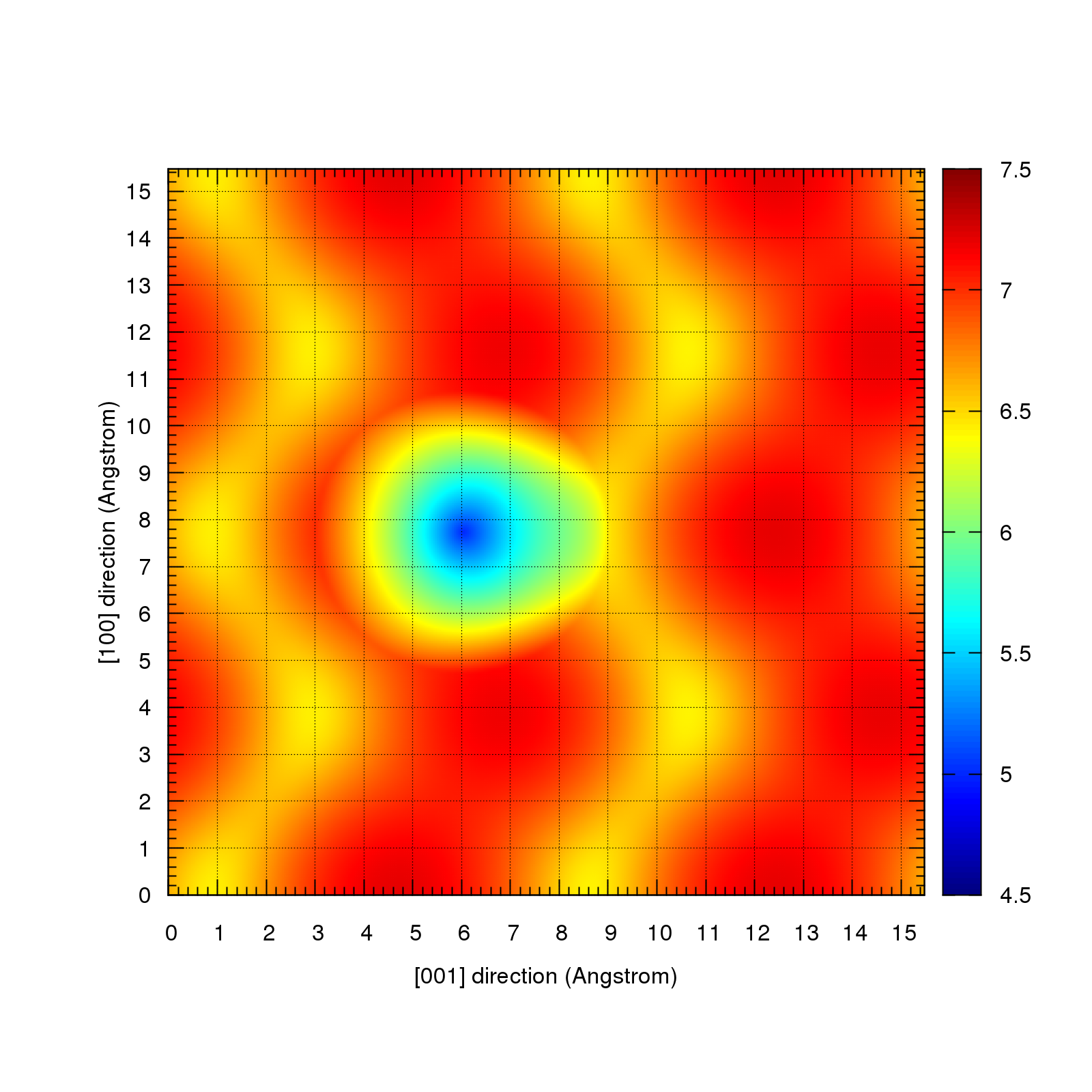
STM叠加-特定范围线性拟合
把PLOTCON-CO和
PLOTCON-Clean进行叠加,中心原子设为CO的坐标,拟合半径r=3,拟合方法为
- 对于
0 < distance < 3的点,电流的取值为$I = {distance \over r}I_{clean} + (1 - {distance \over r})I_{CO} $ - 对于
distance > 3的点,电流的取值为$I = I_{clean} $
使用方法为,将plot_stm.py、PLOTCON-CO和
PLOTCON-Clean
放在一个文件夹下面,在终端下输入
python plot_stm.py PLOTCON-CO PLOTCON-Clean 3
脚本文件如下
#!/usr/bin/env python
#   plot_stm.py
#   2015-11-07
#   Zeyuan Tang

import numpy as np
import math
import os
import subprocess
from sys import argv

"""
center_file = "PLOTCON-CO"
out_file = "PLOTCON-Clean"
radius = 3
"""

center_file = argv[1]
out_file = argv[2]
radius = float(argv[3])
center_point = [6.0339, 7.7357]
output_file = "temp.txt"
result_file = "temp-result.txt"

def write_in_numpy(center_file, out_file, center_point, radius, output_file):
    center_array = np.loadtxt(center_file)
    out_array = np.loadtxt(out_file)

    result_array = []
    index = 0
    for line in out_array:
        distance = math.sqrt((line[0]-center_point[0])**2 + (line[1]-center_point[1])**2)
        if distance <= radius:
            # Important!
            center_line = center_array[index]
            line[2] = (distance/radius)*line[2] + (1-(distance/radius))*center_line[2]

            result_array.append(line)
            index += 1
        else:
            result_array.append(line)
            index += 1

    np.savetxt(output_file, result_array, fmt="%.4f %.4f %8e")

def modified_output(out_file, modified_file):
    f = open(out_file, "r")
    new_file = open(modified_file, "w")
    for line in f:
        new_file.write(line)
        if line.split(" ")[0] == "15.4715":
            new_file.write("\n")
    f.close()
    new_file.close()

write_in_numpy(center_file, out_file, center_point, radius, output_file)
modified_output(output_file, result_file)

plot = open("gplot.plt", "w")
plot.write("#!/bin/bash \n")
plot.write("set terminal pngcairo enhanced color solid lw 2 font 'Helvetica, 25' size 1600,1600 \n")
plot.write("set output 'PLOTSTM.png' \n")
plot.write("set grid \n")
plot.write("set key font 'Helvetica, 20' nobox noreverse noinvert \n")
plot.write("set xlabel '[001] direction (Angstrom)' \n")
plot.write("set ylabel '[100] direction (Angstrom)' \n")
plot.write("set xrange[0:15.4715] \n")
plot.write("set yrange[0:15.4715] \n")
plot.write("set xtics 1 \n")
plot.write("set ytics 1 \n")
plot.write("set mxtics 5 \n")
plot.write("set mytics 5 \n")
plot.write("set palette defined (0 0.0 0.0 0.5,")
plot.write("1 0.0 0.0 1.0,")
plot.write("2 0.0 0.5 1.0,")
plot.write("3 0.0 1.0 1.0,")
plot.write("4 0.5 1.0 0.5,")
plot.write("5 1.0 1.0 0.0,")
plot.write("6 1.0 0.5 0.0,")
plot.write("7 1.0 0.0 0.0,")
plot.write("8 0.5 0.0 0.0) \n")
plot.write("set pm3d map interpolate 2,2 \n")
plot.write("splot 'temp-result.txt' u 1:2:3")
plot.close()

subprocess.call(["gnuplot", "gplot.plt"])
subprocess.call(["rm", output_file, result_file, "gplot.plt"])
最终得到的STM图如下